Entropy Elasticity of Gaussian Polymer Chains
High molecular weight polymers that exhibit rubber-like behavior are known as elastomers. Above the glass transition temperature, the rubber-like polymers are in a liquid-like state and the mer or repeat units change their position readily and continuously due to Brownian motion. Thus, each polymer chain takes up random conformations in a stress-free state.
When considering conformations of many ideal rubber-like chains or conformations of a single chain at different times, the random distribution of the chain ends can be described by a Gaussian function. The probability of a chain having its ends separated by a distance R(N) is given by
![]()
where R0(N) is the average of the squares of the end-to-end distances of the relaxed chain composed of N repeat units.
External Force Acting on the Polymer Chain End
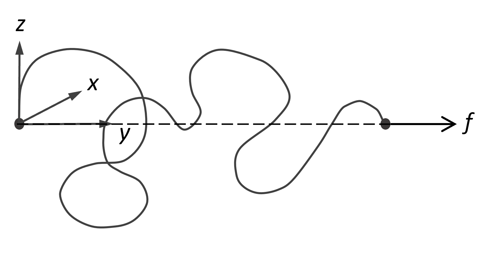
A tensile or shear deformation induces larger chain dimensions and a reduction in free energy F, which in turn, leads to a retractive force f which is consistent with entropy elasticity:
![]()
![]()
where Ω ∝ P(N,R) is the number of possible chain conformations of a polymer chain with an (extended) end-to-end distance R.(1)
In the case of an ideal chain, R0 is independent of temperature because all possible random arrangements are equally likely. Then the retractive force f in the equation above arises solely from an entropic mechanism, i.e., from the tendency of the chains to adopt conformations of maximum randomness, and not from any energetic preference for certain conformations over others. The retractive force f is then directly proportional to the absolute temperature T.
The equations above are only applicable to chains with short end-to-end distances, r2 ≈ Nl2, and in first approximation for distances less than about one-third of the length of fully stretched chains (contour length). For chains with larger end-to-end separation we have to choose a different model. It can be shown that P(N,R) can be estimated with the inverse Langevin function of R/Nl (3,4):
L-1(R / Nl) = L-1(ν) and L(v) = coth(ν) - 1/ν
where L-1 denotes the inverse Langevin function. An expansion of this relation in terms of R/Nl yields4,5
ln P(N,R) = const. - N [3/2·(R/Nl)2 + 9/20·(R/Nl)4 + 99/350·(R/Nl)6 + ...]
whereas the Gaussian distribution leads to the expression ln P(N,R) = const. - N 3R2/2Nl2. With
f = - kT ∂ln P(N,R) / ∂R
the equation above may be written as
f = 3kT/l [(R/Nl) + 3/5·(RNl)3 + 99/175·(R/Nl)5 + ...]
This equation predicts a steeper rise in tension when the chain end separation is R/Nl > 0.3 , i.e., when the chain becomes nearly taut (see figure below).
Tension–Displacement Relation for Freely Jointed Chain
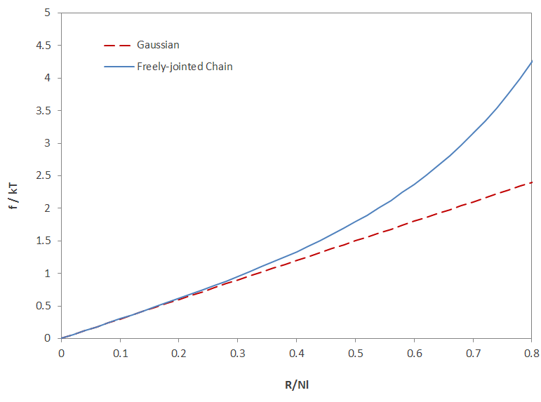
The equations above describe the retractive force of a single chain on extension. For small extensions, the retractive force is proportional to R, that is, a Gaussian chain behaves like a Hookean spring.
References and Notes
For an ideal chain, where there are no enthalpic interactions between the repeat units, the total number of states of a chain with fixed ends, R= |r1 - r2|, is given by Ω1 = ZnP(R,N), where Zn is the total number of conformations. Then the total number of conformations of a chain with an end-to-end distance R is Ω2= Zn 4πR2 P(R,N).
For real polymers, consisting of a large number N of primary valence bonds along the chain backbone, each of length l, the true end-to-end distance is noticeably larger than that of a Gaussian chain
R02 = C∞Nl2
where the coefficient C∞ is the so called characeteristic ratio which is the ratio of the unperturbed mean square end-to-end distance to the mean-square end-to-end distance of the freely jointed chain.
C∞ is found to vary from 2 to 10, depending on the chemical structure of the molecule and also on the temperature, because the energetic barrier to bond rotation is more easily overcome at higher temperatures. C∞1/2l can be regarded as the effective bond length of the real chain, which is a measure of the stiffness of the polymer.- W. Kuhn, Kolloid-Z. 101, 248 (1942),Kolloid-Z. 76, 258 (1936)
- P.J. Flory, Principles of Polymer Chemistry, New York 1953
The Langevin function L(x) = coth(x) -1/x was named after Paul Langevin. For small x values, this function can be approximated by a (truncated) Taylor series: L(x) = x/3 - x3/45 + 2x5/945 - x7/4725, wheares the inverse Langevin function L-1(x), defined on the open interval (−1, 1), can be approximated by L(x) = 3x + 9x3/5 + 297x5/175 + 1539x7/875 + ...